roXefeller
Hazard to Others

Posts: 463
Registered: 9-9-2013
Location: 13 Colonies
Member Is Offline
Mood: 220 221 whatever it takes
|
|
Green's function
Has anyone ever tried using the Green's function treatment to solve an unsteady ode? Usually I would step it out either with an Euler or runge kutta
method, or implicitly if it wasn't too bad. But I was looking at this method below for solving the generalized problem of Lu=f where f is a forcing
function, L is a generalized operator like species concentration or electronic linear equations, and u is the unsteady response. I don't know how I
know I'm capturing all the eigenvector space for creating the Green's function. Imagine a 1D unsteady ode of a chemical species concentration in a
tube with boundary conditions for the species on each end. The ode tells me how the species migrates from the boundaries onto the domain. Can anyone
think through this problem with me?
https://en.m.wikipedia.org/wiki/Green's_function
|
|
|
wg48
National Hazard
Posts: 821
Registered: 21-11-2015
Member Is Offline
Mood: No Mood
|
|
Quote: Originally posted by roXefeller  | Has anyone ever tried using the Green's function treatment to solve an unsteady ode? Usually I would step it out either with an Euler or runge kutta
method, or implicitly if it wasn't too bad. But I was looking at this method below for solving the generalized problem of Lu=f where f is a forcing
function, L is a generalized operator like species concentration or electronic linear equations, and u is the unsteady response. I don't know how I
know I'm capturing all the eigenvector space for creating the Green's function. Imagine a 1D unsteady ode of a chemical species concentration in a
tube with boundary conditions for the species on each end. The ode tells me how the species migrates from the boundaries onto the domain. Can anyone
think through this problem with me?
https://en.m.wikipedia.org/wiki/Green's_function |
I have used the impulse response of analogue and digital electronics, mechanical and optical systems to solve the response of a system to a time
dependent input both analytically and numerically (simulation).
I am not very experienced in partial differential equations or eigenvectors. You appear to use different nomenclature than I am unfamiliar with, but
perhaps I can help if you expand on the problem. Are you trying to determine the concentration of something diffusing along a tube as a function of
time and position along the tube given the concentration at one or bothends of the tube as functions of time?
Do you have MathCad?
|
|
|
roXefeller
Hazard to Others
Posts: 463
Registered: 9-9-2013
Location: 13 Colonies
Member Is Offline
Mood: 220 221 whatever it takes
|
|
I know I can skin this cat in other ways. I'm hoping to learn a new tool that might assist me when those other methods are unusable. And the subject
of species diffusion is simple enough to discuss.
Let's posit that I have a one-end-closed tube which is long and narrow enough to be one dimensional. Initially it has a steady concentration of
oxygen and argon. Then I introduce new unsteady boundary conditions at the open end which induce a diffusion of additional argon or oxygen into the
tube. So I can solve this easily with the unsteady diffusion equation, and let's assume I have done this already in numerous cases with different
initial conditions and boundary conditions. Assume now that I have these cases, which were integrated numerically, stored in array structures over
the dimension and time.
The generalization of the problem says that I know f and u of the equation Lu=f where u=u(x,t) is the argon concentration at location x and time t,
and f=f(t) is the concentration at the open end at time t . And over the space of (u,f) pairs that I've previously computed, I can quantify either L
or its eigenvector decomposition. From this decomposition then I can create a numerical surface G(x,s) that will let me solve for a new u using a new
f which I haven't previously considered. That's the problem I'm hoping to consider. In some cases the Green's function convolution is cheaper to
solve than the integration, which is the motivation to this method.
|
|
|
wg48
National Hazard
Posts: 821
Registered: 21-11-2015
Member Is Offline
Mood: No Mood
|
|
If the equations describing diffusion are inhomogeneous linear differential equations then the supposition principal applies. Which means if you know
the green functions of u(x,t) ( u(x,t) of an impulse f(t)) then the u(x,t) can be calculated by convolving the green functions with the particular
f(t) for which you require the u(x,t) .
Your question was “I don't know how I know I'm capturing all the eigenvector space” How does that relate to my first paragraph?
My understanding is that the eigenvector space can be frequency space ie the FT of the Green functions. Is that what you mean?
I think about these types of problems in terms of input, output and transfer functions of networks. f(t) is the input, the output is u(x,t) and the
transfer function is the impulse response of the network ie the frequency response or what you call Green functions.
|
|
|
roXefeller
Hazard to Others
Posts: 463
Registered: 9-9-2013
Location: 13 Colonies
Member Is Offline
Mood: 220 221 whatever it takes
|
|
One technique for developing the Green's function surface is to establish the space of normalized eigenfunctions or vectors of the operator L. Then
the summation of X*X'/m will approach the Green's function where X is an eigenvector X' is the conjugate eigenvector and m is the eigenvalue of that
eigenvector. It is similar to FT since it has a spectral quality about it. You can see this better on the wiki page. I'm not good with LaTex
formatting, but I should look it up.
I look at the eigenvector decomposition because an array structure of concentrations u and inputs f should make for a matrix L operator.
|
|
|
aga
Forum Drunkard
Posts: 7030
Registered: 25-3-2014
Member Is Offline
|
|
Go LaTeX !
Those formulae are beautiful.
Edit:
$$e=mc^2$$
$$f(x)=\integ{2x^3+x^2+1}$$
Bugger. I forgot too.
[Edited on 21-6-2018 by aga]
|
|
|
roXefeller
Hazard to Others
Posts: 463
Registered: 9-9-2013
Location: 13 Colonies
Member Is Offline
Mood: 220 221 whatever it takes
|
|
Ok so Green's function G is the sum over the eigenvector/values for
\begin{aligned}
n&=1\ldots\infty\\
G(x,x^\prime) &= \sum \frac{\Psi_n^\dagger(x)\times\Psi_n(x^\prime)}{\lambda_n}
\end{aligned}
Not bad for an iPad. Still can't figure out the inline code.
|
|
|
aga
Forum Drunkard
Posts: 7030
Registered: 25-3-2014
Member Is Offline
|
|
Impressive !
No idea what it means, but it looks super skookum.
How would you apply it to the gases-diffusing-in-a-tube problem ?
|
|
|
roXefeller
Hazard to Others
Posts: 463
Registered: 9-9-2013
Location: 13 Colonies
Member Is Offline
Mood: 220 221 whatever it takes
|
|
Well as I was reading and thinking about the method I realized that the currently posited tube is still a homogeneous boundary value problem, Lu=0.
So let's add a twist on it. Let's make the tube out of a slightly permeable ceramic that allows argon to pass. But due to variability in sintering
the it permeates differently along its points. And it is unsteady still. So the problem is Lu=h, where h=h(x,t). f(t) is still for the tube
boundary condition.
\begin{aligned}
u(x,t) &= \int G(x,x^\prime,t,t^\prime)h(x^\prime,t^\prime)dx^\prime dt^\prime
\end{aligned}
|
|
|
wg48
National Hazard
Posts: 821
Registered: 21-11-2015
Member Is Offline
Mood: No Mood
|
|
Apparently diffusion in 1D can be modelled by a RC transmission line. Which means a step function increase concentration at the open in will propagate
down the tube with some velocity and be reflected at the closed end. So the concentration at any point along the tube will be the sum of the forward
and reflected waves. So in the frequency domain that means the response is in infinite series of pole and zeros separated by a frequency interval that
is a function of the diffusion length of the tube. My limited understanding of eigenvectors suggests they represent the poles and zeros. So the number
of vectors you require is determined by how a high a frequency you want to consider.
A leaky tube could probably be modelled as a series R and parallel R and C transmission line which would add decaying terms (tanh) to the wave
propagation.
So what is the relation between poles/zeros and eigenvectors??? Can we explore that please.
[Edited on 23-6-2018 by wg48]
Borosilicate glass:
Good temperature resistance and good thermal shock resistance but finite.
For normal, standard service typically 200-230°C, for short-term (minutes) service max 400°C
Maximum thermal shock resistance is 160°C
|
|
|
roXefeller
Hazard to Others
Posts: 463
Registered: 9-9-2013
Location: 13 Colonies
Member Is Offline
Mood: 220 221 whatever it takes
|
|
I agree that it is similar to an RC in that it is first order with time
\begin{aligned}
\frac{\partial u}{\partial t} + k\frac{\partial^2 u}{\partial x^2} &= F\\
\end{aligned}
But the reflection behavior sounds much more wavelike and I would think requires inductance and a second order in time to act like a wave.
\begin{aligned}
\frac{\partial^2 u}{\partial t^2} + k\frac{\partial^2 u}{\partial x^2} &= F\\
\end{aligned}
When I've used Fourier methods to solve the diffusion equation in the past, the time solution from separation of variables was always a decaying
exponential and the spatial variable was the solution requiring a sum of sinusoids that were spatially periodic. Their magnitudes were always linked
to the exponential and decreasing.
\begin{aligned}
u &= e^{-\lambda t}\sum ( A_n sin\frac{n\pi x}{L} +B_n cos\frac{n\pi x}{L} )\\
\end{aligned}
|
|
|
wg48
National Hazard
Posts: 821
Registered: 21-11-2015
Member Is Offline
Mood: No Mood
|
|
Its standard nomenclature in transmission line theory to refer to the movement of disturbances as the propagation of a wave and to describe what
happens at a change in impedance as reflection (the closed end of the tube is modelled as an open circuit).
Your are correct that an infinitesimal section of the transmission line is a first order RC. Do you consider two such sections cascaded to be first
order?
What about an infinite number cascaded sections would that still be first order?
A first order system cannot have a phase shift greater than 90deg while a transmission line can have any phase shift.
Yes the response of a transmission line (linear system) to a step input can be can be calculated be summing the response to each frequency component
(sin wave) of the step input. That’s true of the spatial function too.
I made an error. The transfer function (frequency response) at a point along the tube is an infinite series of poles and zeros but they are separated
by an interval that is a function of the distance from that point to the closed end of the tube not the length of the tube because there is no
reflection at the driven end.
I should also add that due to the frequency dispersion of a RC transmission the step at the input is distorted as it propagates down along the line.
Apparently a RC transmission line is an accurate model of 1D diffusion in a tube or putting it an other way the equations are identical in both cases.
If you want the complicated details you can search for “transmission line model of diffusion” and “telegraphic equations”
For example https://en.wikipedia.org/wiki/Telegrapher%27s_equations.
PS I will attempt to explain the the last part of your last post later. The equations in your last post were missing when I first viewed it.
Borosilicate glass:
Good temperature resistance and good thermal shock resistance but finite.
For normal, standard service typically 200-230°C, for short-term (minutes) service max 400°C
Maximum thermal shock resistance is 160°C
|
|
|
roXefeller
Hazard to Others
Posts: 463
Registered: 9-9-2013
Location: 13 Colonies
Member Is Offline
Mood: 220 221 whatever it takes
|
|
I must admit my laziness. While I've had formal education for poles and zeros, they aren't a technique I use and so I'm quite rusty. The last time I
was trying to solve for transmission line behavior (January last) I took the shortcut and time stepped it with RK4 or euler implicit. I know other
valid theories exist for it, but I also wanted to know the transient behavior during a capacitive discharge into the transmission line and a nonlinear
load at the end.
I keep wondering if I can study this diffusion problem with a blocky discretization, such that it is easy to visualize. But I wonder if the
discretization error would be a stumbling block before I even got started. I need to look for a paper that I've heard about on this topic.
Attachment: greensfunctions-logan.pdf (539kB)
This file has been downloaded 723 times
Attachment: Greensfunctionchapterpdf (95kB)
This file has been downloaded 606 times
|
|
|
roXefeller
Hazard to Others
Posts: 463
Registered: 9-9-2013
Location: 13 Colonies
Member Is Offline
Mood: 220 221 whatever it takes
|
|
| Quote: |
So what is the relation between poles/zeros and eigenvectors??? |
Bear with me, I'm rusty on my transfer functions. This is all probably review for you but I'll provide my understanding and maybe you can fill in
where I'm lacking, I'm certainly not telling you what is what.
What we are looking for with a pole/zero analysis is the root locus where we seek to know the roots of the transfer function. We want to know the
roots because they are the real/imaginary/complex power of the exponential. And that exponential is based on the trial solution to the equation. If
I were to take the same ode and attempt an alternate solution using separation of variables, I would achieve an eigenvalue problem where the
derivative of the eigenfunction needs to be a multiple of the same function Df=lamba f. So what is the physical reality of the eigenfunction? In one
way, its a coordinate transformation to diagonalize a system of equations to become a number of independent equations. They don't need solved as a
system. It can also be seen as a basis for a function space where all possible solutions are linear combinations of all of the functions. In the
idea of transfer function roots, the eigenfunctions are the assumed exponential function while the eigenvalue is the root that defines the behavior of
the function.
Obviously two ways to core the apple and get to the same answer. Why would I choose one over the other. The root locus method, which I'm assuming is
why you are interested in poles and zeros, provides a rich understanding of where the eigenvalues/roots will appear. It provides a strong intuition
on this. But in it you consider the eigenfunction, e^x, only in passing and as a carrier of the more important root.
In eigenfunction/eigenvector analysis it isn't usually assumed that the exponential is the answer. Often it isn't, depending on the boundary
conditions, like with the erf function, and something more complex is expressed along with a number that is considered spectrally. So I would choose
an eigenfunction decomposition when I want to understand the building blocks of the possible solutions. You mentioned the tanh function. Is that
because it was derived from two eigenfunctions that produced the hyperbolic exponentials? From reflective boundary conditions on the far end?
I just read about using the step function with ode integration to derive the Green's function. I should consider that as something to compare the
eigenvector combination.
|
|
|
battoussai114
Hazard to Others
Posts: 235
Registered: 18-2-2015
Member Is Offline
Mood: Not bad.... Not bad.
|
|
Some words of caution:
First, I'm no mathematician, my background is in engineering and I haven't used linAlg for years.
Second, I actually left this post written in the quick reply box for a few days before posting, so it might not be relevant anymore.
My understanding regarding how many eigenfunctions you would need to find so that you can span all your space is as follows:
Assuming that my rusty linear algebra still applies you'd have infinite eigenfunctions, since any scalar multiple of an eigenvalue or function
would still be a a valid one for your transformation, only by adding some sort of condition like a bounded space you'd limit the actual number of
eigenvectors/functions that are possible. The thing is how many associated eigenvalues you can find for your problem, which I think is a value that
has an upper bound depending on the size of your transformation matrix though it can be any natural number from zero to this upper bound. You'd be
trying to find enough so that your eigenfunctions can satisfy the requisite that they form a basis for your space.
For eivenvectors this would be as simple as proving they're linearly independent, for eigenfunctions the requisites may be a little more complex,
can't really say I remember that.
So the first step would probably be build your eigenvalue problem and see how many roots your characteristic polynomial has, from there you'd see how
many forms your eigenfunctions can take based on each eigenvalue you got. Then you'd check wether these functions form a basis for your space and
finally integrate over them to get your answer.
I feel like this would be all nice and good as long as your model is well formulated. It still leaves one loophole, this whole crap I wrote basically
dances around the problem of figuring how many eigenvalues you'd need to figure the problem out by assuming the ones you will find actually are
enough. I fell that might not really be the case though. Which would leave us with one important question: how would you determine the dimensions of
your function space so that you can figure how many eigenfunctions you need in order to span it all? Maybe getting some clues from your modeling? I
sincerely have no clue...
Batoussai.
|
|
|
wg48
National Hazard
Posts: 821
Registered: 21-11-2015
Member Is Offline
Mood: No Mood
|
|
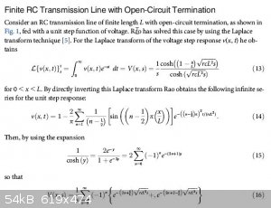
roXefeller:
While swotting up on RC transmission lines I found a paper that calculates the step response of a open ended RC transmission line using the diffusion
equation. See http://journals.plos.org/plosone/article/file?id=10.1371/jou...
Below is a screen copy of the relevant equations. The Laplace transfer function is shown on the first line. The s roots of the denominator are the
poles and the s roots of numerator are the zeros for a given position.
I am unable to equate your x,t solution with the one. shown. But neither one has the form I was expecting. In general I thought transmission line
problems have hyperbolic functions in them because of the way amplitude varies along a lossey transmission line and a section of a transmission line
with discontinuities at the end can have repeating poles or/and zeros unless damping factor is greater than critical ie two solutions depending on
the damping factor which I neglected.
Yes you can use the root locus method to adjust the stability, bandwidth or step response, but the position of the poles and zeros also give insight
in to the form of the transfer function and its response.
battoussai114:
Unfortunately I am no mathematician either. Most of my maths are vaguely connected patches of knowledge from my old engineering life. Your post was
helpful in helping me link Laplace to eigenvectors I am still digesting it.
PS: Its probably obvious that the Laplace transfer function is the right hand term of the first equation less the 1/s which is the step function.
[Edited on 26-6-2018 by wg48]
[Edited on 26-6-2018 by wg48]
Borosilicate glass:
Good temperature resistance and good thermal shock resistance but finite.
For normal, standard service typically 200-230°C, for short-term (minutes) service max 400°C
Maximum thermal shock resistance is 160°C
|
|
|
roXefeller
Hazard to Others
Posts: 463
Registered: 9-9-2013
Location: 13 Colonies
Member Is Offline
Mood: 220 221 whatever it takes
|
|
As for pde classifications, the transmission line is hyperbolic as you said. That class, like a traveling fluid wave, admits a solution that isn't
necessarily informed by the boundary conditions, unless they are within the zone of influence. Interestingly, in compressible fluid flow we can see
supersonic flow where the characteristic lines all point backwards, leaving the forward field completely unaware of the approaching wave. The
diffusion problem is a parabolic type of pde, which like the elliptic type, requires solutions that are simultaneously informed by the boundary
conditions. Examples of other elliptic equations are potential fluid flow and material elasticity. There might be some cases in electromagnetics,
like electric field potential, but that's only speculation on my part. The term that causes a parabolic to become hyperbolic is the time derivative.
For rigid body or electric circuits, this requires an inertial term (mass or inductance) which seeks to maintain a velocity. No such quantity exists
in heat diffusion because it would violate the laws of thermodynamics. Hence time derivatives limit out at the first order derivative.
Do you really leave inductance out of your transmission line problems? Or is that just a case of implied vernacular?
|
|
|
roXefeller
Hazard to Others
Posts: 463
Registered: 9-9-2013
Location: 13 Colonies
Member Is Offline
Mood: 220 221 whatever it takes
|
|
So I had a chance to write down the finite difference equations to convert the partial operators into linear algebra form.
\begin{aligned}
u_t + k u_{xx} &= h (x,t) \\
u_t &= \frac{u_i^{n+1}-u_i^n}{\Delta t}\\
u_{xx} &= \frac{u_{i+1}^{n+1}-2u_i^{n+1}+u_{i-1}^{n+1}}{\Delta x^2}\\
\frac{u_i^{n+1}-u_i^n}{\Delta t} + k\frac{u_{i+1}^{n+1}-2u_i^{n+1}+u_{i-1}^{n+1}}{\Delta x^2} &= h_i^n\\
\end{aligned}
This is obviously with an implicit euler integration. The thing to note is the stencil, where the n index of h is related to n and n+1 (possibly
even n-1 in general depending on any other schemes to approximate the first partial derivative), and the same for each i index related to i, i-1, and
i+1. If u and h are both spatio-temporal where column n is the instantaneous solution at time n, then they are both matrices. The L operator
operates on a matrix and produces a matrix, but in this way it isn't standard linear algebra since that operates vector by vector and this stencil has
to operate between columns. No L would take the 4th order form:
\begin{aligned}
L_{jkmn}u_{mn} &= h_{jk}
\end{aligned}
Or multilinear algebra. Sadly after Einstein, it has only had sporadic work done because of the computational cost until most recently with big data
mining. I'm currently reading some recent articles to find what modern mathematicians are writing about multilinear spaces.
|
|
|
wg48
National Hazard
Posts: 821
Registered: 21-11-2015
Member Is Offline
Mood: No Mood
|
|
| Quote: Originally posted by roXefeller |
Do you really leave inductance out of your transmission line problems? Or is that just a case of implied vernacular? |
An odd question. What I can say is it depends on the details of the particular problem and what I was trying to achieve with the analysis and or
simulations
When dealing with audio signals or slow digital transitions signals the resistance capacitance and inductance of the interconnects (transmission
lines) between components on a printed circuit board could be assumed to have no resistance, capacitance or inductance because the propagation time
was small compared to the period of the maximum signal frequency. Longer connections would be modelled as a lumped capacitance ignoring only the
inductance. These days with GHz bandwidth semiconductors even interconnects on the same board have to be treated as transmission line with L and C.
On one project with miles of coax even the dispersion had to be considered.
Signal lines within in a small integrated circuit that are very short in electrical length compared to the signal wave length can be analysed with
sufficient accuracy by assuming the inductance is zero. Similar to the example I gave.
In a different scenario helical resonators with sufficiently large end capacitive load are analysed by ignoring the distributed capacitances and
resistance ie a Tesla coil secondary with a capacitive top load significantly larger than the distributed capacitance of the coil.
In short you ignore the terns you can and don’t when you cannot. But you must have known that already. Well you did ask.
Borosilicate glass:
Good temperature resistance and good thermal shock resistance but finite.
For normal, standard service typically 200-230°C, for short-term (minutes) service max 400°C
Maximum thermal shock resistance is 160°C
|
|
|
MJ101
Hazard to Self
Posts: 82
Registered: 14-6-2018
Member Is Offline
Mood: Always Sunny
|
|
@roXefeller: I haven't tinkered with this stuff in many years. 
Maybe this might help?
http://citeseerx.ist.psu.edu/viewdoc/download?doi=10.1.1.445...
https://www.researchgate.net/figure/The-influence-of-the-str...
@wg48: As you pointed out. In some cases, it matters. Otherwise, what would we do with all of those cute little ferrite beads
and nifty snubbers. 
|
|
|
wg48
National Hazard
Posts: 821
Registered: 21-11-2015
Member Is Offline
Mood: No Mood
|
|
| Quote: Originally posted by roXefeller | So I had a chance to write down the finite difference equations to convert the partial operators into linear algebra form.
\begin{aligned}
u_t + k u_{xx} &= h (x,t) \\
u_t &= \frac{u_i^{n+1}-u_i^n}{\Delta t}\\
u_{xx} &= \frac{u_{i+1}^{n+1}-2u_i^{n+1}+u_{i-1}^{n+1}}{\Delta x^2}\\
\frac{u_i^{n+1}-u_i^n}{\Delta t} + k\frac{u_{i+1}^{n+1}-2u_i^{n+1}+u_{i-1}^{n+1}}{\Delta x^2} &= h_i^n\\
\end{aligned}
This is obviously with an implicit euler integration. The thing to note is the stencil, where the n index of h is related to n and n+1 (possibly
even n-1 in general depending on any other schemes to approximate the first partial derivative), and the same for each i index related to i, i-1, and
i+1. If u and h are both spatio-temporal where column n is the instantaneous solution at time n, then they are both matrices. The L operator
operates on a matrix and produces a matrix, but in this way it isn't standard linear algebra since that operates vector by vector and this stencil has
to operate between columns. No L would take the 4th order form:
\begin{aligned}
L_{jkmn}u_{mn} &= h_{jk}
\end{aligned}
Or multilinear algebra. Sadly after Einstein, it has only had sporadic work done because of the computational cost until most recently with big data
mining. I'm currently reading some recent articles to find what modern mathematicians are writing about multilinear spaces. |
I think you are talking about state space techniques or it’s related to state space technique. It’s used in control theory, target tracking, and
error correction in for example inertial navigation system. Lots of papers and books have been written on the subject.
Borosilicate glass:
Good temperature resistance and good thermal shock resistance but finite.
For normal, standard service typically 200-230°C, for short-term (minutes) service max 400°C
Maximum thermal shock resistance is 160°C
|
|
|