mayko
International Hazard

Posts: 1218
Registered: 17-1-2013
Location: Carrboro, NC
Member Is Offline
Mood: anomalous (Euclid class)
|
|
on the distribution of r**2 values (a retraction)
I recently called bullshit on a graph posted by the most recent PhD incarnation (worst Doctor ever!!), specifically on the basis that I doubted
that the reported coefficient of determination (r**2) of 0.000 was realistic.
After posting, I realized ........ that I was going entirely on intuition and I didn't actually know what the distribution of r**2 was for
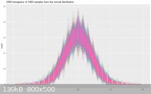
correlations of random noise! It's easy to find out though. First, I generated 1000 runs of noise from a normal distribution, each the same length as
the one PhD showed us (217 points):
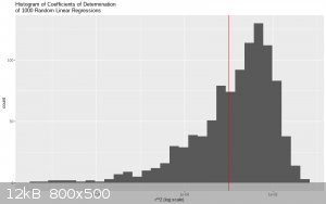
Next, I added a dummy variable and ran a linear regression on each one. Then I gathered the r**2 values from those regressions and I will be damned if
a full third of them weren't smaller than 0.001 and a quarter of them smaller than 0.0005!
| Code: |
smol (<0.001)          verysmol (<0.005)
 FALSE:632       FALSE:747
 TRUE :368       TRUE :253
|
Here is a histogram of the distribution with the 0.001 threshold marked with a red line (note the log scale):
Every day is a winding road!
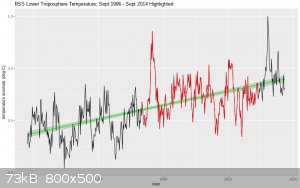
So then I had to go ahead and check; I downloaded the data cited ( RSS_Monthly_MSU_AMSU_Channel_TLT_Anomalies_Land_and_Ocean_v03_3.txt; here: http://data.remss.com/msu/monthly_time_series/ ) and I couldn't believe my eyes but when the regression results came it was the flattest line
drawn through the noisiest data:
| Code: |
> lm(global ~ otherDate, data = RSS %>% filter(date>ymd(19960901)) %>% filter(date < ymd(20141001))) %>% glance()
# A tibble: 1 x 11
    r.squared adj.r.squared sigma statistic p.value    df logLik   AIC   BIC deviance df.residual
        <dbl>         <dbl> <dbl>     <dbl>   <dbl> <int>  <dbl> <dbl> <dbl>    <dbl>       <int>
1 0.000000353      -0.00465 0.169 0.0000758   0.993     2   78.4 -151. -141.     6.17         215
> lm(global ~ otherDate, data = RSS %>% filter(date>ymd(19960901)) %>% filter(date < ymd(20141001))) %>% tidy()
# A tibble: 2 x 5
  term         estimate std.error statistic p.value
  <chr>           <dbl>     <dbl>     <dbl>   <dbl>
1 (Intercept) 0.197       4.42      0.0445    0.965
2 otherDate   0.0000192   0.00220   0.00871   0.993
|
An r**2 of 0.000000353 and an effect size of 0.0000192 C/year, or 0.00192 C/century. What a world.
Anyway the point here is to share the null r**2 distribution since I don't think I'd actually seen it before and to concede that this was in fact the
garden-variety grift:
| Quote: |
* subset the data in a very particular way (usually, by sticking the record-breaking 1998 El Nino at the start of the time series to make the ensuing
regression to the mean tank the trend)
* fit a regression to data, albeit not necessarily an appropriate one
* accurately report the results
* fail to mention the false-positive rate of the hiatus- or cooling-detection method employed
* ignore or misinterpret statistical significance as needed
|
Here is the RSS data as a whole, with the cherrypicked region highlighted in red. A linear fit gives a warming rate of 1.3C/century. (also, this is
what an r**2 of 0.44 looks like.)
(mods feel free to append to the trash thread)
al-khemie is not a terrorist organization
"Chemicals, chemicals... I need chemicals!" - George Hayduke
"Wubbalubba dub-dub!" - Rick Sanchez
|
|
|
clearly_not_atara
International Hazard
Posts: 2693
Registered: 3-11-2013
Member Is Offline
Mood: Big
|
|
mayko, I think you're missing something quite obvious, and I hope you're not too embarrassed when you notice it.
For a correlation with zero slope, r^2 is ALWAYS zero!
The reason is that r denotes the correlation between z-scores. That is, one standard deviation of increase in the independent variable produces r
standard deviations of increase in the dependent variable. For complex statistical reasons, |r| < 1 always. But if the slope of the correlation is
zero, obviously any increase in the independent variable produces no increase in the dependent variable, and r = 0 trivially.
The extension to the linked graph is immediate. Since the graph was created by picking a time period in which the long-run change in temperatures was
zero, of course it has an r^2 of zero.
What does that prove, exactly? Nothing. What it proves is that r^2 is not a useful descriptive statistic for a correlation with zero slope. (Instead,
use the standard deviation of the dependent variable to describe the correlation.)
Something tells me that someone had intended to use r^2 = 0 as a "proof" that the correlation was strong. This is exactly backwards. r^2 = 1 is a
strong correlation. r^2 = 0 means no correlation. But again, this is meaningless at zero slope.
[Edited on 04-20-1969 by clearly_not_atara]
|
|
|
mayko
International Hazard
Posts: 1218
Registered: 17-1-2013
Location: Carrboro, NC
Member Is Offline
Mood: anomalous (Euclid class)
|
|
"I wouldn't say I've been missing it, Bob..." 
It's definitely true that a regression with a slope of zero has an r**2 of zero, but not a single one of the thousand fits to random data DID have a
slope of zero. None had a slope with absolute magnitude smaller than 10^-6 in fact, and they were centered ~ 8*10^-4
Remember, part of my suspicion WAS the reported slope of 0.00 C/century, and this numerical sim seems to give weak justification to that suspicion.
If I scale the slope up two orders of magnitude (mirroring the scaling of a C/year rate into a C/century rate), less than 7% have a scaled slope
smaller that 0.01 and less than 4% have a scaled slope smaller than 0.005. So yes, it is a *little* unusual to see an effect size that small in a
truly random data set, but you are right that the effect size has also been driven downward by deliberate selection.
| Code: |
 linear_fits %>% rowwise()%>% tidy(model) %>% ungroup() %>% filter(term=="coord") %>% select(c(dist,estimate)) %>% mutate(mag=abs(estimate), scaled_mag=100*abs(estimate), smol=scaled_mag < 0.01, verysmol=scaled_mag<0.005) %>% summary()
dist        estimate               mag              scaled_mag           smol
 1      :  1   Min.   :-3.738e-03   Min.   :3.329e-06   Min.   :0.0003329   Mode :logical
 2      :  1   1st Qu.:-6.385e-04   1st Qu.:3.479e-04   1st Qu.:0.0347894   FALSE:931
 3      :  1   Median : 8.803e-05   Median :7.370e-04   Median :0.0736952   TRUE :69
 4      :  1   Mean   : 6.421e-05   Mean   :8.609e-04   Mean   :0.0860938
 5      :  1   3rd Qu.: 8.363e-04   3rd Qu.:1.244e-03   3rd Qu.:0.1243669
 6      :  1   Max.   : 3.302e-03   Max.   :3.738e-03   Max.   :0.3738221
 (Other):994
  verysmol
 Mode :logical
 FALSE:967
 TRUE :33
|
My interpretation was that they were treating the r**2 like a significance measure, and then confusing "failing to reject the null hypothesis" with
"affirming the null hypothesis". But maybe they just got really excited by all the zeros and wanted to emphasize the zero-ness of it all xD
al-khemie is not a terrorist organization
"Chemicals, chemicals... I need chemicals!" - George Hayduke
"Wubbalubba dub-dub!" - Rick Sanchez
|
|
|
Gearhead_Shem_Tov
Hazard to Others
Posts: 167
Registered: 22-8-2008
Location: Adelaide, South Australia
Member Is Offline
Mood: No Mood
|
|
This is what honest people do when they make a mistake: they tell others about it, even when the mistake is subtle or slightly arcane. Well done,
mayko.
|
|
|
|