woelen
Super Administrator

Posts: 7977
Registered: 20-8-2005
Location: Netherlands
Member Is Offline
Mood: interested
|
|
Experiment with algebraic integers
I expect all of you know the concept of integer numbers (..., -3, -2, -1, 0, 1, 2, 3, 4, ....) and rational numbers (1/2, 7/8, -12/25, etc.).
Rational numbers can be regarded as solutions of linear equations ax + b = 0, for integer a and b. If a is equal to 1 or -1, then the solution is an
integer. For each rational number x, there is a smallest number d, such that d*x is an integer (e.g. for x=2/7, the value of d is equal to 7, and d*x
equals 2). The number d is called the denominator of the rational number.
Sums, differences and products of integers are integers as well (in mathematical terms, the set of integers, with addition and multiplication is
called a ring, but this is not important for appreciating the nice things, which follow).
The nice thing is, that the concept of integers and rational numbers can be generalized. For instance if we take the equation a*x^2 + b*x + c = 0,
with integer a, b, c, such that this equation cannot be reduced to a product of two linear factors with integer coefficients, then the solutions of
these equations are called algebraic numbers of degree 2. If a equals 1 or -1, then the solutions are called algebraic integers of degree 2 (the
ordinary integers are algebraic integers of degree 1). In general, if we have an n-th degree equation, with the coefficients of the leading term equal
to 1 or -1, and the equation being irreducible (it cannot be reduced to a product of factors with lower degree and integer coefficients), then the
solutions of that equation are called algebraic integers of degree n. An example is the equation x^3-2 = 0. This has three solutions cbrt(2),
(-1+i*sqrt(3))*cbrt(2)/2, (-1-i*sqrt(3))*cbrt(2)/2. These three solutions all are algebraic integers of degree 3. Here cbrt() is the cubic root and
sqrt() is the square root. The number i is the imaginary number i*i = -1.
These algebraic integers have some very interesting properties and also have many applications in mathematics, number theory and cryptography. What I
wondered about was, how are these numbers distributed over the complex plane? The algebraic integers of degree 1 all are on the real line, at 0, -1,
1, -2, 2, -3, 3, etc. The algebraic integers of degree 2 mostly are on the real axis, but there also are complex ones. Algebraic integers of degree 3
for really interesting patterns in the complex plane.
I wrote a program, which determines algebraic integers of degree 1 up to and including degree 9, with coefficients of a maximum given height (either
positive or negative). This is not really trivial, especially determining whether an equation is irreducible or not is not that easy. I used a sieve
process, using lower degree factors to check the irreducibility of higher degree equations.
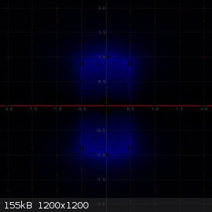
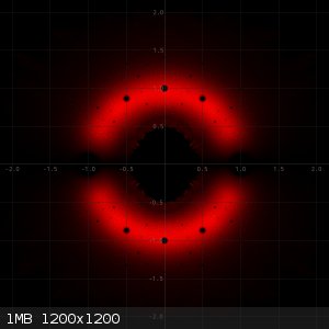
The first picture below is a picture of algebraic integers of degree 1 (the green dots), degree 2 (the red dots) and degree 3 (the blue dots). I took
the degree 1 equations of maximum height 50, the degree 2 equations with maximum height 30, and the degree 3 equations with maximum height 25. The
leading term always is kept equal to 1 (otherwise it is not an algebraic integer). The reducible equations I discarded. Solutions from these already
are covered in lower degree equations.
Below follows a picture of the degree 1, 2, 3 algebraic integers. One dot for each of the values found:
Next, a picture follows when degree 4 algebraic integers are added with maximum height 20. Yellow dots are added for degree 4 algebraic integers.
An also a file with 5-th degree algebraic integers of maximum height 10. A somewhat darker cyan/dull blue dot is added for each algebraic integer of
degree 5.
Finally, I also created a picture, which adds all algebraic integers of degree 6 with maximum height 8. For these I used another visualization method.
All algebraic integers heat a pixel somewhat. All pixels start from black and the higher a pixel's value, the hotter it is displayed (from black to
white through red, orange, yellow).
All pictures show really interesting patterns for the distribution of these algebraic integers. The complete set of algebraic integers of any degree
is dense over C, but the distribution is not uniform at all. Whether a set of algebraic integers of a specific degree is dense in C I do not know.
E.g. the set of algebraic integers of degree 2 is not dense in C, there are only discrete red dots in the picture. It is dense in R though. For degree
3, things become already much more itneresting and really wonderful patterns emerge.
I was surprised by these really interesting distributions and wanted to share these with you. I'm not able to explain these patterns, I'll do some
deep diving into that. Maybe I find interesting results.
Anyway, algebraic numbers, algebraic integers and the related concept of number fields is quite interesting. A nice introductory read about the
subject, which is easy to understand for someone with mathematics at starting university level, or maybe even some advanced high school level, is
available here: https://www.math.leidenuniv.nl/~evertse/dio17-3.pdf
A final remark: view the pictures at exactly 100% scale (1200x1200 pixels), so that pixels are not blurred. This gives the best view of the intricate
patterns.
[Edited on 6-2-24 by woelen]
|
|
|
woelen
Super Administrator
Posts: 7977
Registered: 20-8-2005
Location: Netherlands
Member Is Offline
Mood: interested
|
|
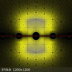
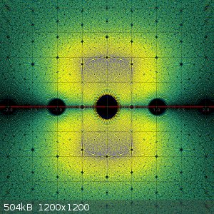
In the following three pictures I made heat plots of
1) All zeros of all reducible polynomials of degree 9 and maximum height of absolute value of coefficients equal to 3.
2) All zeros of all irreducible polynomials of degree 9 and maximum height of absolute value of coefficients equal to 3.
3) All zeros of all polynomials of degree 9 and maximum height of absolute value of coefficients equal to 3.
Zeros on the real axis are not plotted, that's just a nearly uninterrrupted white line.
 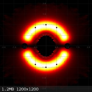 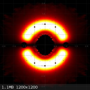
The last image is the combined heat map of the two previous ones. You can see that when reducible polynomials are taken into account, then many very
hot small dots are added. This can be explained, because many reducible polynomials of maximum height 3 will have the same small factor with small
coefficients and hence zeros of such small factors frequently occur, leading to heating of the same pixel over and over again.
Computing all of these pictures took approximately 5 minutes on a single core of an i7-13700 running at 5000 MHz or so. The right picture requires
computing the zeros of appr. 40 million 9th degree polynomials. The middle picture takes about 30 million polynomials and the left picture takes a
little over 10 million polynomials. So, in total well over 80 million 9th degree polynomials in 5 minutes.
[Edited on 21-2-24 by woelen]
|
|
|
clearly_not_atara
International Hazard
Posts: 2696
Registered: 3-11-2013
Member Is Offline
Mood: Big
|
|
It's an interesting finding, but it's important to remember two things:
- sums and products of algebraic integers are algebraic integers
- sums and products of algebraic integers with normal integers are algebraic integers of the same degree
The second property is easily proven; the first property is proven by a similar argument that requires some clever linear algebra. From the second
property, we find that the set of algebraic integers is translationally invariant with period 1 and scale invariant as well. So these localized
structures appear as the density of algebraic integers whose minimal polynomial has small coefficients.
It's important to remember that it isn't possible to define a distribution like "a uniform distribution across all natural numbers". Consequently, the
"density" of algebraic integers only exists so far as we choose a normalizeable distribution which is usually induced by a normalizeable distribution
on Z.
It looks like you've chosen something resembling a uniform distribution across coefficients in {n | n in Z, n < M} for some limit
M. Maybe try with normally distributed coefficients?
[Edited on 04-20-1969 by clearly_not_atara]
|
|
|
j_sum1
Administrator
Posts: 6229
Registered: 4-10-2014
Location: Unmoved
Member Is Offline
Mood: Organised
|
|
Lovely work woelen.
I had not come across algebraic integers before. At first blush I thought you were talking about gaussian integers... but that is a different thing
again.
Writing some code to solve that many polynomials is no trivial thing. I think this is outstanding.
I am not 100% certain what you mean by "height". I might have to read your explanation again.
I vividly recall the moment when I discovered that the rationals were dense on R but not continuous. (This was independent of any mathematic tuition i
was receiving, which was nice.) It seems that we have a similar pattern occurring on C with these sets of numbers.
A possible extension might be to allow complex coefficients of your polynomials -- ie, Gaussian integers. I expect that the results would be various
rotations of what you already have, but there may be some other patterns emerge.
Another thing I would be interested in is subsets of the numbers found. What happens if some coefficients remain fixed and others are varied. I know
there have been interesting studies on solutions to equations of the form x^5+ax+b=0.
Anyway. Beautiful images and a very interesting study.
Edit
I think it is interesting how there is a depletion zone around lower order numbers which lowers the density of higher order numbers in that vicinity.
(There is probably a less awkward way of saying this, but hopefully I am clear enough.)
[Edited on 23-2-2024 by j_sum1]
|
|
|
woelen
Super Administrator
Posts: 7977
Registered: 20-8-2005
Location: Netherlands
Member Is Offline
Mood: interested
|
|
@clearly_not_atara: The properties you give indeed are true, but things are even better.
Any monic polynomial (i.e. a polynomial whose term with highest degree has coefficient equal to 1), which has coefficients, which are algebraic
integers, has zeros, which also are algebraic integers.
For any algebraic number there is a smallest ordinary integer, such that the product of the algebraic number and that integer is an algebraic integer.
This smallest number can be regarded the "denominator" of the algebraic number. It is a generalization of the concept of denominators in ordinary
fractions.
Yet another very interesting thing, which I found numerically, and which I later also found explained in algebra texts is that the set of reducible
polynomials in Z[X] has density 0.
The experiments I did are quite complicated, because simply solving polynomial equations is not the complete story. In most of my pictures I only want
to plot zeros of irreducible polynomials (over Z). Reducible polynomials can be written as a product of two lower degree polynomials, but when such
polynomials are solved numerically, then one does not easily find the degree of each of the zeros. The degree of a zero may be lower than the degree
of the polynomial you have. The last three pictures show the effect of taking reducible polynomials as well.
I did not really take a distribution of polynomials, I took ALL polynomials not exceeding a certain height of a given degree.
The height of a polynomial is the largest of the absolute values of all coefficients. E.g. the height of x^3 + 5*x - 7 is 7, the
height of x^7 - 4*x^5 + 5*x^3 - 4*x - 4 is 5.
The latest set of plots uses monic polynomials of degree 9 with height not exceeding 3. I.e. all coefficients, except the one for x^9 can have values
equal to -3, -2, -1, 0, 1, 2, 3, hence 7 possibilities. There are 7^9 (which is well over 40 million) such polynomials. Of these, well over 10 million
are reducible.
I am working on a set of web pages about polynomials and polynomial-like functions and the distribution of zeros of them. One of these is about
algebraic integers. Then I'll also give some theory.
[Edited on 23-2-24 by woelen]
|
|
|
Rainwater
National Hazard
Posts: 800
Registered: 22-12-2021
Member Is Offline
Mood: indisposition to activity
|
|
You should meet up with 3blue1brown. Lots of good videos about math with explanations that i can understand
"You can't do that" - challenge accepted
|
|
|
Metacelsus
International Hazard
Posts: 2531
Registered: 26-12-2012
Location: Boston, MA
Member Is Offline
Mood: Double, double, toil and trouble
|
|
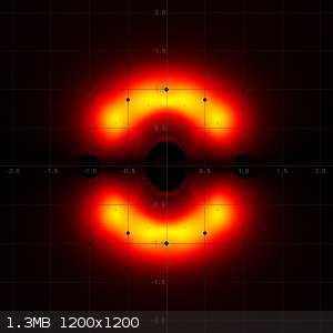
What are the small black circular regions of lower density?
Grant (3blue1brown) is a super cool guy, I met him once at a conference. This definitely looks like something that would interest him.
|
|
|
woelen
Super Administrator
Posts: 7977
Registered: 20-8-2005
Location: Netherlands
Member Is Offline
Mood: interested
|
|
@Rainwater: I did not know 3blue1brown, but now that I have watched a few videos from him, I must say that I am impressed. He uses beautiful
animations and has a very pleasant way of telling things. the relaxing music in his videos also helps. It does not distract one from the subject, but
it makes listening to what is told much easier. Very well done.
@Metacelcus: The small black regions of low (or even zero density) are small areas around zeros of polynomials of lower degree, which are factors of
reducible polynomials of the degree under investigation.
Just to give an example: -3 - 3*x + 3*x^2 - x^3 - x^5 + 3*x^6 + 3*x^7 - 2*x^8 + x^9 can be written as (-1 + x)(1 + x + x^2)(3 + 3*x - 3*x^2 + 4*x^3 +
3*x^4 - 2*x^5 + x^6)
This polynomial has 9 zeros, one of them being 1 (a zero of degree 1), two of them being -0.5 + 0.5*sqrt(3) and -0.5 - 0.5*sqrt(3) and six of them
being the zeros of the sixth degree factor, which cannot be further reduced. Around 1, -0.5 + 0.5*sqrt(3) and -0.5 - 0.5*sqrt(3) there are areas of
much lower density. Around the zeros of the sixth degree polynomial, the density also is lower, but the effect is less pronounced. That's what I
demonstrate with the three pictures in the post of 21-2-2024.
Another interesting observation is that a polynomial of a given height H (in this case H equals 3), if it is reducible, can have factors with a higher
height. The above-mentioned sixth degree factor has height 4. Things can be even more extreme. For 9-th degree polynomials with height 3, the largest
possible height for one of the factors is 16. For example, the polynomial (3 -2 3 -3 -3 -2 -3 3 -3 1) can be written as (1 1) (1 1 1) (3 -8 13 -16 11
-5 1). Here , (.. .. ..) is a shorthand notation for a polynomial with coefficients starting from the constant term to the term with the highest
power, e.g. (2 1) stands for 2+x and (4 -3 2 1) stands for 4-3*x+2*x^2+x^3. As I am dealing with monic polynomials in all my computations (remember,
we're doing algebraic integers) the last coefficient in the (.. .. ..) notation always is equal to 1.
[Edited on 25-2-24 by woelen]
|
|
|
Metacelsus
International Hazard
Posts: 2531
Registered: 26-12-2012
Location: Boston, MA
Member Is Offline
Mood: Double, double, toil and trouble
|
|
I understand why the points 1, -0.5 + 0.5*sqrt(3) and -0.5 - 0.5*sqrt(3), etc have low density, but I'm surprised that the regions around
them also have low density, in a vaguely hexagonal pattern. Why would this be the case?
|
|
|
woelen
Super Administrator
Posts: 7977
Registered: 20-8-2005
Location: Netherlands
Member Is Offline
Mood: interested
|
|
Actually, the points at 1, -0.5 + 0.5*sqrt(3) and -0.5 - 0.5*sqrt(3) have zero density if only irreducible 9th-degree polynomials of a given maximum
height are considered. If all 9th-degree polynomials of a maximum given height are considered, then these points have very high density. This is
because these numbers are zeros of polynomials of lower degree (degrees 1 and 2) and there are many reducible 9-th degree polynomials with linear or
quadratic factors, having these numbers as zeros.
The fact that the areas around these points have lower density is much harder to explain. In order to explain, I have to digress a little. Let's first
talk about irreducible polynomials of degree larger than 1 with integer coefficients. Such polynomials do not have integer roots (otherwise they would
be reducible and they would have a linear factor (x-n), with n the integer root). These polynomials can have roots, which are close to integer values.
How close these roots can be to integer values, depends on the height of the polynomial. The higher the height, the closer one can get to an integer
root. E.g. the polynomial x^2 + 9999999999999999*x + 10000000000000000 has two real roots, one of them very close to -1 (actually, very close to
10000000000000000/9999999999999999, but not exactly equal to that. This polynomial also has very large height (this is 10000000000000000). Now imagine
that you have polynomials with an height at most equal to 3. You will see that now, you cannot get really close to -1 or 1. For how close one can get
to an integer for irreducible polynomials with integer coefficients, there are known bounds, which are functions of the height and degree of the
polynomial.
A similar thing also exists for the more general case of algebraic integers. Instead of linear factors (for normal integers), we now talk about
low-degree factors, which can have real or complex zeros, but around these zeros there also is a certain area, which cannot be reached for higher
degree polynomials with a given height. The larger the height, the smaller the areas, which cannot be reached, but the density of these areas still
remains lowers. The actual pattern for higher and lower densities is amazingly complex and I think that the normalized density plot for the height
going to infinity is a fractal. Drawing it is not easy, it requires solving many many polynomial equations. For a large height, the number of
polynomial equations grows really rapidly with increasing degree.
|
|
|
|